Calculating existing LTV is a simple equation. You have the purchase history, you add it up, you have a number. LTV prediction is a different problem: it estimates what a customer will spend in a future window, from signals available today, before most of that spending has happened. That gap between what a customer has done and what they will do is where media buying decisions, retention budgets, and acquisition ceilings actually get set.
A study from Bain & Company found that in financial services, a 5% increase in customer retention drives more than a 25% increase in profit (Bain, Prescription for Cutting Costs). Peter Fader, who did much of the foundational academic work on customer lifetime value at Wharton, used it to forecast Wayfair's revenue years forward.
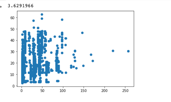
We built one for a large mobile app that monetizes through in-app purchases and media buys across five paid channels. It predicts 60-day customer spend within 3.62%. For you this could be as simple as taking data you already have and plugging it into one of our popular algorithms built for any business model with customers, and in this article we’ll walk through modern approach options, and the path we took to reach that accuracy in production.
✂️ Definition
What is LTV prediction?
Lifetime value (ltv) prediction is the use of statistical or machine learning models to estimate how much revenue a customer will generate over a future time window, based on signals available now. It differs from LTV, which sums revenue a customer has already produced. A production LTV prediction model takes customer and cohort features (acquisition channel, demographics, early purchase behavior, engagement events), learns the relationship between those features and eventual spend, and outputs a predicted value for a defined horizon such as 60, 90, or 180 days. Accuracy is usually reported as mean absolute percentage error (MAPE) at a given horizon, and under 10% at one year is a commonly cited benchmark.
What LTV Prediction Predicts, and Over What Window
Despite the word lifetime, the evaluated horizons are almost always fixed. Businesses predict at window intervals, usually 30, 60, 90, 180, or 365 days, because that is what the available history supports and what planning cycles need. When you see an accuracy figure quoted for an LTV model, the horizon it was measured at matters as much as the number itself. A 5% error at 30 days and a 5% error at 365 days are not comparable achievements.
Before predicting anything, you need to settle how your customer lifetime value calculation works on the history you already have, and there are three ways depending on what your data supports.
Customer level. You have purchase amounts and dates per individual customer, so you compute LTV per person. This is what you want, and it is what makes per-customer prediction possible.
Aggregate level. You only have totals, so you divide revenue in a period by customers in that period and work with an average revenue per customer. Coarse, but workable when per-user data does not exist.
Cohort level. You can group customers by acquisition month, channel, or product category even if you cannot resolve individuals, so you compute LTV per cohort. This is the level most media buying decisions actually get made at, which is why cohort prediction is often more useful than per-customer prediction even when both are possible.
Predicting forward from any of those splits into two families of data models. Statistical models assume purchase behavior follows a known probability distribution and fit its parameters to your data. Machine learning models make no such assumption and instead learn the relationship between customer features and eventual spend from examples.
The Three Model Families, and How to Pick One
Building data models for LTV comes down to three families, and almost every system in production is one of them. The choice is driven less by what is most sophisticated and more by what your data can support and what the output has to do.
Statistical models need the least: purchase amounts and dates, nothing else. They fit fast, they run in a notebook or a spreadsheet, and they give you a defensible baseline within days. Gradient boosting is the workhorse and the right default for most teams, because tabular customer data with mixed categorical and numeric features is exactly what it was built for. Deep learning earns its keep when you have high-dimensional behavioral signals, event streams, browsing sequences, in-app actions, that resist hand-engineering into features, or when you need a custom loss function that a boosting library will not give you cleanly.
One rule that saves projects: run the statistical baseline first even if you intend to ship machine learning. It takes a week, it lets you verify initial assumptions about how your customers actually buy, and it answers the question that matters most, which is whether a predictive signal exists in your data at all. If a well-fit BG/NBD model cannot beat a naive average by a meaningful margin, a neural network is not going to rescue you, and you have learned that for the price of a week rather than a quarter.
Model family
Data it needs
Output
Uncertainty
Reach for it when
Statistical (BG/NBD, Pareto/NBD, Gamma-Gamma)
Purchase amounts and dates
Expected transactions and value per customer
Credible intervals from the fitted distribution
You need a baseline this month, or you are testing whether signal exists at all
Gradient boosting (LightGBM, XGBoost, CatBoost)
Tabular features: channel, geo, device, demographics, early behavior
Point prediction per customer or cohort
Only with a distributional loss such as ZILN or Tweedie
This is the default. Mixed feature types, moderate data, production in weeks not months
Deep learning (DNN with ZILN, sequence models)
Everything above plus event streams and behavioral sequences
Full predicted distribution, not just a point
Native: ZILN returns a mean and a standard deviation
High-dimensional behavior resists feature engineering, or you need a custom loss
Not sure which family your data actually supports?
Tell us what you have: how much history, at what granularity, and what decision the prediction has to feed.
We will tell you what is buildable and what is not before anyone writes code.
Statistical Baselines: BG/NBD, Pareto/NBD, and Gamma-Gamma
These models split the problem in two. A counting model such as BG/NBD or Pareto/NBD predicts how many purchases a customer will make, treating purchase timing as a Poisson process and customer dropout as a probability that resolves after each transaction. A value model, usually Gamma-Gamma, predicts what each of those purchases will be worth. Multiply the two and you have predicted LTV. The only inputs are recency, frequency, and monetary value, all derivable from a transactions table.
For every ecommerce client we work with, we fit these before touching machine learning. They train in seconds, the parameters are interpretable enough to sanity check against what the business already believes about its customers, and they establish the number any later model has to beat. If you are starting from nothing, the maintained Python implementations of these models are a better first stop than the older packages most tutorials still point at.
Modern Machine Learning for LTV Prediction
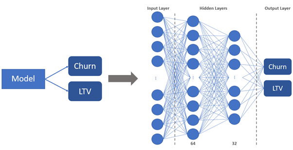
Deep neural network to create an LTV prediction and customer churn
If you want a reasonable place to start on an LTV prediction model in 2026, gradient boosting on tabular customer features is where we see the best out of the box results. LightGBM, XGBoost, and CatBoost all handle the job well. CatBoost tends to need less preprocessing when high-cardinality categoricals like campaign ID or affiliate ID carry a lot of the signal, which for acquisition data they frequently do.
Treat these options as starting places rather than a ranking. A retailer with eight years of clean per-customer transaction history and a mobile app with two weeks of post-install signal are not solving the same problem, and the approach that wins on one can lose badly on the other. Data shape and prediction windows decide this more than the model itself does, so fit two or three candidates and let your own data analysis guide the best approach forward. What we consistently find is that the loss function and data analysis move accuracy more than the library choice does.
What actually goes into the model
Feature engineering decides more of the outcome than architecture does, and for LTV the most relevant data falls into four groups. RFM aggregates come straight off the transactions table: recency, frequency, monetary value, and tenure. Early-window behavior is where most of the signal lives for day-N prediction, and it is what lets you estimate a new user's value long before they have any purchase history, meaning session and engagement data such as first-session depth, events fired on day 1, day 3, and day 7, and the timing and size of the first purchase. Acquisition metadata covers channel, campaign, creative, affiliate, geography, and device, which are all categorical and often high cardinality, and that is the specific case CatBoost handles better than the alternatives. Then derived timing features, of which the gap between first and second purchase is usually among the strongest single predictors you will find, because a customer who comes back quickly behaves very differently from one who takes three months.
One practical trick if your boosting library does not give you a custom loss cleanly. Train two models instead of one: a classifier that predicts whether the customer returns at all, and a regressor trained only on customers who did return, predicting how much they spent. Multiply the two outputs. That is the same decomposition ZILN performs internally, built from standard components, and it gets you most of the benefit without writing a custom objective. It also has a diagnostic advantage, since you can see immediately whether your error is coming from misjudging who returns or from misjudging how much they spend.
Why mean squared error is the wrong loss for LTV
LTV prediction is a regression problem, so the reflex is mean squared error. MSE fails here for two specific reasons, both identified clearly in Wang et al's work at Google.
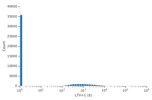
The first is zero inflation. In most apps and catalogs only a minority of users ever become paying users at all, and a large share of those buy once and never return, so their label is zero. But that zero means "did not come back," not "came back and spent nothing," and MSE cannot tell those apart. When most of your labels are zeros of the first kind, the model spends its capacity learning to predict zero.
The second is the heavy tail. Revenue distributions are dominated by a small number of very high spenders, and those data points sit orders of magnitude away from the median. Because MSE squares the error, those outliers generate enormous gradients, and the model contorts itself trying to fit customers who represent a tiny fraction of the population. The result is a model that is bad at whales and, because it spent everything trying, also bad at everyone else.
Zero-inflated lognormal loss, and the three numbers it returns
A huge reason we use ZILN is its built for the key issue in pLTV: most customers are one time purchasers with zero LTV, skewing the dataset
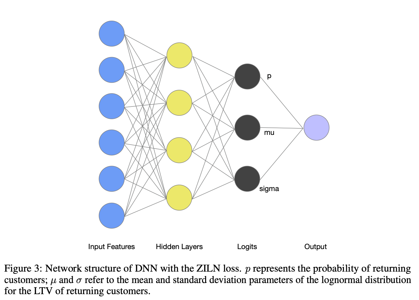
The fix is a loss function that treats LTV as two problems at once. Zero-inflated lognormal loss, introduced in A Deep Probabilistic Model for Customer Lifetime Value Prediction, pairs a classification term for whether a customer returns at all with a regression term that models spend as a lognormal distribution, which is naturally shaped for heavy tails.
In a neural network this shows up as an output layer with three units rather than one. The first produces p, the probability the customer makes another purchase, through a sigmoid. The second produces the mean of the spend distribution for returning customers, with identity activation. The third produces its standard deviation, through softplus to keep it positive. Two shared hidden layers of 64 and 32 units sit underneath, learning a representation that serves both the classification and the regression task. On the Kaggle acquire-valued-shoppers dataset, ZILN beat MSE by 11.4% relative on the Gini coefficient for classifying returners, and cut decile-level MAPE by 68.9%.
That third output is the most useful of the three. A point estimate tells you a cohort is worth $42. A distribution tells you it is worth $42 with a standard deviation of $18, which is a completely different input to a bidding decision. If you are allocating marketing spend against channel-level acquisition ceilings, bidding on a lower confidence bound rather than a mean is the difference between a target you can defend and one that blows up the first time a cohort underperforms.
Behavioral embeddings as features
The sequence of products a customer browses carries real signal about what they will eventually spend. High-value customers look at expensive, less popular items; low-value customers cluster around discounts. The problem is dimensionality: with 85,000 catalog items and 12.5 million customers, the space of possible browsing sequences is far too large to hand-engineer into features. Chamberlain et al solved this in Customer Lifetime Value Prediction Using Embeddings by learning low-dimensional customer embeddings with skip-gram negative sampling, defining a customer's context as other customers who viewed the same products at around the same time. A context of 11 customers worked best. Their baseline was a regression random forest on handcrafted features drawn from demographics, purchase history, returns, and product data, and it reached a Spearman rank correlation of 0.46 between predicted and actual LTV. Adding the customer embeddings as an extra feature produced measurable AUC uplift on the companion classifier, with optimal embedding lengths between 32 and 128.
That paper contains an insight worth carrying forward on its own. They treated a customer with zero purchases in the last year as churned, which means churn classification and LTV prediction are the same model looking in two directions. If you are already building a churn prediction model, most of the feature engineering transfers directly.
Where the research is now
Deep networks for LTV are well established at this point. Pollak's eyewear retail study compared a fully connected network of five dense ReLU layers against a Pareto/GGG statistical model on the same sales data, and reported 94.6% accuracy for the network against 88.6% for Pareto/GGG. Two things are worth taking from that. The deep model won, and the statistical baseline was already close enough to be useful, which is the argument for fitting one before you build anything larger.
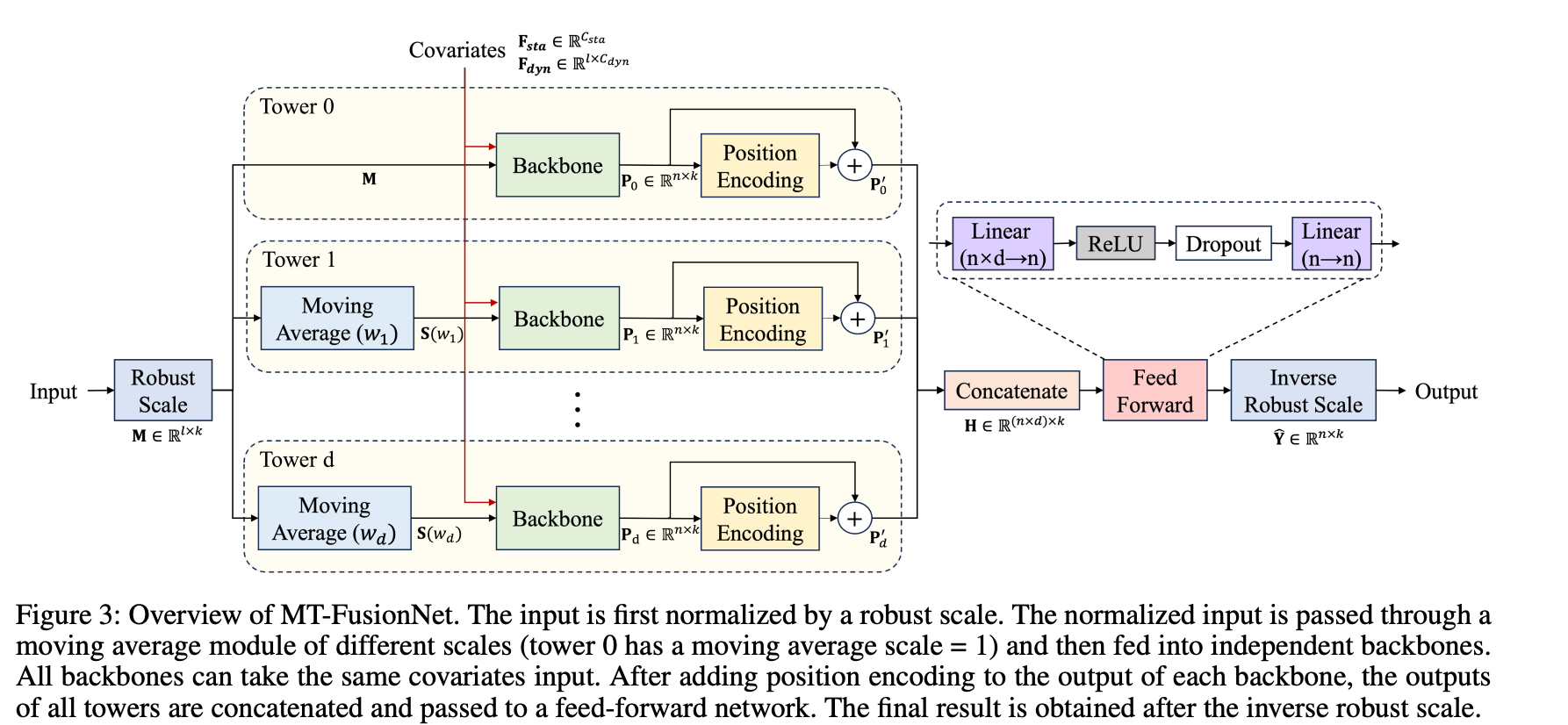
More interesting is where the problem has moved since. ByteDance published TTF, a trapezoidal temporal fusion framework for LTV forecasting in Douyin, accepted to the AAAI 2026 IAAI track, and it names the problem most production teams actually face.
Channel-level LTV is not one time series, it is many unaligned ones, because each acquisition channel starts on a different date and has a different amount of history. It is also what they call a short-input long-output problem: you have days of signal after a user installs and you need to forecast months forward. Their framework handles the misalignment explicitly and reports MAPE reductions of 4.3% and 3.2% against the models it replaced in production. If you are forecasting LTV per channel to set media budgets, or to see which marketing campaigns prove profitable long before the revenue actually lands, that is the shape of your problem, and it is worth knowing that the research has caught up to it.
Where LLMs Fit in LTV Prediction, and Where They Do Not
This question comes up on every scoping call now, and the answer has two halves that get conflated constantly.
A large language model is the wrong tool to make the prediction. LTV prediction is numerical regression over structured tabular data, and gradient boosting and ZILN-based networks win at it precisely because they exploit numerical structure. Paste a customer's transaction history into a chat model and ask what they will spend next quarter and you will get a fluent, plausible number. What you will not get is calibration, an uncertainty estimate, a probability that the customer returns at all, or any way to hold the result to a MAPE target. LLMs are non-deterministic, so you can’t trace the logic for how the model reached that output. They just generate the next best token, not compute math values.
Where language models do help is upstream, turning unstructured signal into features the tabular model can use. Three patterns are worth knowing.
Text embeddings as features. Support tickets, product reviews, chat transcripts, and survey responses become dense vectors that feed into the model alongside conventional features. This is the Chamberlain idea generalized: any high-dimensional behavioral signal can become a low-dimensional feature.
Summarization into structured fields. A messy event stream gets condensed by a language model into a handful of structured attributes, which is often more tractable than engineering those attributes by hand from raw logs.
Free-text classification into cohort labels. Where behavioral signals arrive as unstructured text, a model can bucket them into categories that become categorical features.
A Production Build: LTV Prediction for a Mobile App
The client runs a large mobile application monetized through in-app purchases, acquiring users through paid media ad channels like Meta, Google Ads, Microsoft Ads, Taboola, and an email list. Where an app blends purchases with advertising, overall ad revenue belongs in the same target, and the ad revenue generated per user gets forecast alongside purchase spend rather than in a separate model. They needed predicted LTV per segment, broken out by channel, age, gender, and zip code, at several horizons. That one metric feeds a stack of decisions: how much to bid per channel, which in-app purchases to surface to whom, when to surface them relative to a user's purchase pattern, and where in the lifecycle each segment tends to churn so retention effort lands before rather than after. Assessing mobile marketing profitability at the segment level is the job, and mobile marketing prediction models are how you get there without waiting six months for the answer.
Version one did not work, twice
We started where most teams start, with gradient boosting. XGBoost and XGBSEKaplanNeighbors both struggled, because the data was too sparse for specific categories of users. Grouped into cohorts by campaign ID, product ID, and affiliate ID, the model ran an average percent error of negative 24.8%. It was underestimating the client's app revenue by just under a quarter, which is worse than useless for a bidding decision, since it would systematically starve channels that were actually performing.
So we moved to neural networks. They converged, which looked like progress for about a day, and then we looked at what they had converged on. Every customer was getting roughly the average prediction regardless of their features. On individual revenue prediction the numbers were bleak: mean absolute error of 78.32, mean squared error of 9,198.66, and a mean absolute percentage error close to infinite.
A MAPE that large is not a modeling result, it is a signal. Seeing it raised a red flag with our data science team, because a network that refuses to learn anything beyond the mean is usually telling you the features carry no usable relationship to the labels. After two architectures failed the same way, the more likely explanation was that the data needs to be looked at.
Half the training data was garbage
We went back through the dataset the models were training on and found transactions that should never have been in it. Customers with negative revenue, produced by failed refund attempts. Fraudulent and void transactions that the original SQL had not filtered out. Every model we had trained to that point had been fitting a mixture of real purchase behavior and accounting noise.
Working with the client's data team surfaced a description column that let us identify fraudulent and incomplete transactions reliably, along with a few other columns worth feature engineering from. We rewrote the query to exclude them. That filter removed 1.7 million records, roughly 50% of the data we had been training on.
This is the part of the project that mattered most and it involved no machine learning at all. If you take one thing from this section, take that the ceiling on an LTV model is set by whether the training labels represent real purchase behavior, and that a model failing in a strange way is often the cheapest data quality audit you will ever run.
Version two, and the loss function that fixed the tail
With clean data we rebuilt, and the new architecture is simpler than what preceded it. It uses feature component recognizers so the network can train on specific feature groups per user rather than flattening everything into one undifferentiated input, and it replaces the generic regression loss with ZILN.
That swap is the one that made the difference, for exactly the reason described earlier. ZILN stops punishing the network so heavily for missing on large spenders, which frees it to model the average customer properly instead of exhausting itself on the tail. The theory from the Wang paper, deployed against a real revenue distribution.
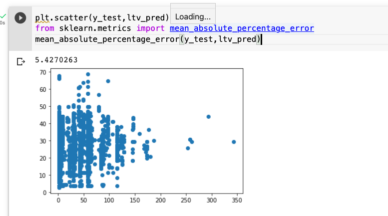
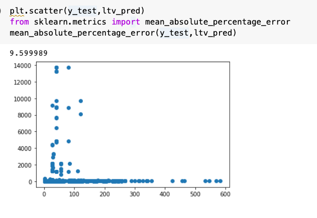
Here is a look at the accuracy difference at different prediction windows:
60 days:
90 days:
180 days:
These are average percentage differences between predicted and actual spend. The dataset carried a lot of outliers, and they account for most of the remaining variance. Some resolved into data collection problems rather than model error, including multiple subscriptions tied to a single account and developer accounts sitting in the production dataset.
What we shipped
The model runs in production, executing daily against new data landing in a Postgres database. It sits behind a training harness on AWS that makes fine-tuning runs fast, which matters because acquisition mix drifts and a model trained on last quarter's channel blend degrades quietly. Incoming customers get bucketed for segmentation through the same categorization architecture we built for Pumice.
Want to know what your data can actually predict?
If you are scoping a predictive LTV model build and want a second opinion on what your data supports, send us the details. Tell us what history you have, at what granularity, and what decision the prediction has to feed. We will tell you what horizon is realistic and where the accuracy ceiling sits before anyone writes a line of code.
Frequently Asked Questions
What does LTV stand for?
LTV stands for lifetime value, sometimes written as customer lifetime value (CLV or CLTV). It measures everything a customer is worth to a company across the whole relationship, mostly revenue but sometimes including indirect value such as referrals. In practice, businesses measure it over a fixed window rather than an actual lifetime.
What is a healthy LTV?
There is no universal number, because LTV is only meaningful against what it costs to acquire the customer. The ratio people watch is LTV to CAC, and a commonly used rule of thumb in subscription and app businesses is that LTV should be at least three times customer acquisition cost, with payback inside twelve months. What counts as healthy varies enormously by margin structure, since LTV is a revenue figure while net profit is what the ratio is really protecting. A business with 80% gross margins can tolerate a much lower ratio than one at 20%. This also heavily depends on your user acquisition model, user behavior, and business model.
What is CLV vs LTV?
They are the same metric. CLV (customer lifetime value), CLTV, and LTV all describe the total value of a customer relationship. Usage varies by industry: mobile and gaming teams tend to say LTV, while retail and subscription analytics tend to say CLV. Predicted versions are written pLTV or predictive LTV, and mean the forecast rather than the historical figure.
Which model should I use for LTV prediction?
Start with a statistical baseline such as BG/NBD paired with Gamma-Gamma, because it takes days and early indicator metrics tell you whether predictive signal exists in your data. Move to gradient boosting with LightGBM, XGBoost, or CatBoost for most production systems, using a loss function suited to revenue data rather than plain mean squared error. Reach for a neural network with ZILN loss when you have high-dimensional behavioral data or need a full predicted distribution rather than a point estimate.
How accurate can LTV prediction be?
It depends heavily on horizon and data quality, so treat any single figure with suspicion unless the horizon is stated alongside it. Under 10% MAPE at one year is a widely cited benchmark. The production system described above reports 3.62% at 60 days and 9.60% at 180 days on the client's own data. Accuracy degrades as the horizon extends, and predictions beyond roughly a year are generally unreliable regardless of the model. Perform ongoing testing to ensure no data drift as overall user behavior changes. The data you have matters, models predict actual outcomes only when the labels/data they learned from were real.
How much data do I need before this works?
You need enough completed windows to learn from, which means historical data from existing customers covering at least the horizon you want to predict. If you are not there yet, run the statistical baseline while gathering sufficient data for a machine learning model. Predicting 90-day LTV requires customers who have been around for 90 days with known outcomes. Total volume matters less than coverage across segments: sparse data within a specific channel or cohort is what breaks models, as it did in the first version of the build above. An experienced data science team is needed to ensure the data quality.